Sunday, March 1, 2015

UAS (Unmanned Aerial System) Mission Planning

Introduction:


Unmanned aerial systems (UAS) are an increasingly prevalent technology that are used to accomplish a wide range of tasks. UAS often get associated with military operations, and often the word "drone" is used incorrectly to describe just one aspect of UAS. As the correct name implies, UAS consist of much more than just an unmanned vehicle. The consist of a platform, or flying device, a sensor, a ground station, radio control, and sometimes autopilot hardware. There are a number of other parts that can be included in UAS depending on it's use.

Not only does the word "drone" have a negative connotation, it also inaccurately describes UAS, implying that they are unmanned, unpiloted robots that operate free of human input. This is false, and the truth is that UAS should always be piloted, whether that be computationally or manually. Best practice for UAS is to have a 3 person team, consisting of a Pilot In Command, who mans the physical controls of the unmanned aerial vehicle (UAV), a Pilot At Controls, who operates sensors, and monitors from a computer, and an engineer/spotter who keeps close watch of the UAV, providing assistance to the PAC and PIC as needed.

UAS often are associated with miliary utility, but it is important to recognise their usefulness in many different situations. In geography, they can be used to assist in research providing aerial imagery, atmospheric monitoring, and many other remote sensing data. It can be a good alternative for other remote sensing utilities because it provides high spatial resolution, rapid results and possibly higher temporal resolution, at a reasonable price.

In this exercise, I looked at some unmanned aerial vehicles, and used a flight simulator software to get a better understanding of the different types of UAV's before acting as a consultant in various situations, recommending a UAS for assistance in various types of research.

Methods:


The first component to this exercise was to use a flight simulator to log flight time on a number of different types of UAV to get to know the strengths and weaknesses associated with each, and ultimately begin to understand some of the possible situations in which they could be used. Doing this, we used RealFlight 7.65 with real UAS remote controllers to try different platforms, utilizing a number of different flight views.

The first platform that I demoed was the Hexacopter 780. This is a multi-rotor platform with 6 propellers that is quite stable, and capable of slow flight speeds, which would allow for high spatial resolution aerial imagery and other remotely sensed data. However, multi-rotor platforms can't manage a very heavy payload, and since they have so many rotors, their battery life time suffers.
I logged around 30 minutes of flight time on the hexacopter on an ocean map with a shipwreck and a number of obstacles. I kept the wind low, as this was my first simulation, and the controls were hard enough as they were. I had five crashes in my 30 minutes of fly time, most of them involving crashes after attempted landings, or collisions with obstacles. 
The next platform I demoed was a fixed wing UAV called the Slinger. Fixed wing platforms are often useful for managing heavy payloads over large study areas. One main detriment to fixed wing UAVs is that they can only slow down to a point (where they will no longer provide lift), and thus cannot achieve as detailed remotely sensed image data as multi-rotored systems.
This is the Slinger, a common fixed wing platform. The controls were very different from the hexacopter, with much higher speed and touchy turns. I demoed this UAV at the Sierra Nevada map, experimenting with heavy winds. It was affected quite significantly by the presence of winds, making potential sampling impossible with adverse conditions. The chase view was the most fun of the different camera views, but I used the fixed view as well, which required some critical thinking about the relative controls. I had 6 crashes in the ~30 minutes that I tested this platform. Most of which were due to my overconfidence, testing maneuvers that would not be acceptable in the field.  
Next, I tested a Quadcopter X platform. This is a multi-rotor platform with just four rotors. The fewer rotors a UAV has, the less stable it is, especially in adverse conditions. However, it can have a longer battery life than multi-rotor platforms with more rotors.
I flew the quadcopter on the junkyard map, for about 30 minutes, experimenting with different views, including the 1st person view. This view allows you to have the perspective as if you were on the nose of the craft. This technology is widely used in real UAS scenarios. I had trouble with the fixed view, crashing four times within the first couple of minutes I attempted takeoff. I also found that succesfully landing the quadcopter was very difficult and required a very light touch with the accelerator joystick. I had a whopping total of 12 crashes in my half hour of flight time. 
Finally, I used the P-51 mustang platform for testing. This is another fixed wing craft, but it is significantly larger than the slinger model, and takes off from a runway on the ground. This model is also gas-powered which allows for longer flights.
I tested the P-51 Mustang on the Junkyard environment, and used the fixed view, chase cam, and cockpit cam for flights. With the Mustang I was able to achieve successful landings! I only had one or two successful landings with the other crafts, but this one I was able to land repeatedly. The controls were less touchy than the slingers', and it flew faster. I only crashed four times in the half hour of flight time logged.  

The final part of this exercise was to use our acquired knowledge to provide consultation for some scenarios created by our professor about possible use of UAS'.

Scenario 1: An atmospheric chemist is looking to place an ozone monitor, and other meteorological instruments onboard a UAS. She wants to put this over Lake Michigan, and would like to have this platform up as long as possible, and out several miles if she can.

Since she wants to cover a large area with a long flight time, this is a good scenario to use a fixed wing craft in. Though I only tested a couple of fixed-wing crafts, I believe that a larger one with a high payload would be advisable to accommodate multiple meteorological instruments. With this in mind, perhaps using a larger, gas-powered UAV would be in her best interest to increase flight time and distance. This would be more expensive, but necessary to accommodate her daunting task of mapping a large chunk of lake Michigan.

Scenario 6: An oil pipeline running through the Niger River delta is showing some signs of leaking. This is impacting both agriculture and loss of revenue to the company.

Depending on the magnitude of the oil leak at hand, a number of different UAS could be used. Since the scenario reads that the pipeline is showing signs of leaking, I will assume that the company is unsure of the problem and its whereabouts. This implies that there is a large area that must be covered to monitor the potential problem, and that sounds best suited for a fixed wing aircraft. Its low flight capabilities, long flight times and speed of data retrieval definitely demonstrate its preferability to satellite imagery, and because of this scenario's large geographic extent, a fixed wing craft is better suited for the task than a rotorred or multi-rotor system.

Conclusion:


This exercise was a valuable introduction to the growing field of UAS technology. These systems facilitate data collection for many different tasks, many of which are directly applicable to geography and geospatial data. Knowing the basics of what these unmanned aerial systems consist of (and what they don't consist of) is important in knowing ways in which we can solve geographic problems. More generally, being able to communicate our knowlege to a potential client is an important skill for workers in the geospatial field, as many clients aren't familiar with the technology. It is important to be able to look at a problem, and find a way to quantify it and collect data.

Sources:

http://www.iupac.org/publications/pac/special/0199/pdfs/engelhardt1.pdf

Friday, February 13, 2015

Development of a Field Navigation Map

Introduction:


This objective of this exercise was to create two navigation maps for use in later field exercises. The maps reference the priory, which is a piece of land owned by UW-Eau Claire that includes over 100 acres of mostly wooded land. It has a number of buildings as well, that are utilized by UW-Eau Claire for academics and a child care program.

See this link for a map referencing the UWEC Priory


It is important to include in navigational maps all of the tools that are necessary to perform the required task. Navigation maps need to be able to be relied upon to represent the real world features to a workable extent, so we had some explicit instructions on what to include.

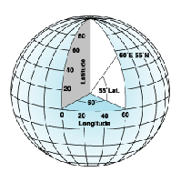
Two different types of coordinate systems were used in this exercise. The first is a geographic coordinate system, which uses a 3D sphere to define locations on earth using degrees. This is what comprises our latitude/longitude system.

This image demonstrates the world as a globe, showing how longitude and latitude values are calculated (with respect to the equator and the prime meridian).

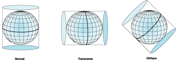
The other type of coordinate system we used is the Universal Transeverse Mercator projected coordinate system. The term projected, means that this model takes a 3D model of the earth, and puts it onto a 2D surface. Because of it's 2D characteristics, projected coordinate systems have constant lengths, angles, and areas- where in a geographic coordinate system, distance these measurements fluctuate based on distance from the equator. However, projected coordinate systems always include a certain degree of error, simply because they aim to represent a 3D feature (the earth) in two dimensions. This results in stretching at the boundaries of the projection, but much research has been done to optimize different projections for use in different geographic areas to reduce error. The projection to be used in this study is Transverse Mercator, which is a cylindrical projection (meaning the earth is essentially placed inside a cylinder and rolled from pole to pole. Thus, the center of the model is the most accurate, with stretching occurring to the sides). Because of this, different zones are defined, with the cylinder touching the globe at various different points- this is the Universal Transverse Mercator System.

This image shows cylindrical projections. Imagine the bold line in the transverse image going down each of those lines of longitude, creating many different "zones" each minimizing the error of the features near it. That is the idea of the UTM system. 


Because geographic coordinate systems are often optimized for smaller scale studies, we were instructed to create two different maps, one using a geographic coordinate system, and the other in UTM. Using this UTM projection, we are able to use meters as our working units, which is often preferable for land surveys.


Methods:


The first component to this exercise was to calculate our pace count. A pace count is a simple but surprisingly valuable tool for use in navigation. With it, you can calculate distance between features without requiring expensive tools like GPS devices, or lasers. For calculating our pace count however, we did use expensive devices. We went out to the parking lot and equipped a couple of students with sonic distance finder, and a laser distance finder. We then had another student walk 100 meters down with a receiver. We marked the exact distance to the 100 meter point, and had each student walk down, counting every time his/her dominant foot fell. I count 65 on my way down, and then 63 on the way back. Averaging these figures gives me a pace count of 64, which I will be using for all further calculations.

With our pace count calculated, the next step was to create our navigation maps. Professor Joe Hupy gave us an introduction to the priory, and instructed us on necessary components for our maps. First and foremost, our maps needed to have a workable grid system that is useful for calculating distance and referencing features. This is achieved through ESRI ArcMap's layout view grids. There are a number of options for the layout and setup of these grids, and it took some fiddling to get a usable grid for reference. For the UTM grid, I used 50 meter increments. For the latitude/longitude map, I used a decimal degrees grid, incrementing by .001 degrees. We were provided with aerial imagery of our study area, within which, we had an area designated for containing the points that we would be surveying later on. All data in this exercise was compiled by Joe Hupy and is located in a departmental priory geodatabase. Other important feature that we included in our navigation maps was the terrain information. Where the aerial imagery provides a good overview of the land surface features, it doesn't show topography very well. Because of this, I included 5 meter contour lines with labels to represent the changes in elevation for use in the field. Also, like any other map, ours were required to include a scale bar, scale text, north arrow, and title- along with relevant metadata (like coordinate system and projection information). The final maps are shown below. They were created in ESRI ArcMap, and finishing touches were added through the use of Adobe Illustrator.

Final map using decimal degrees grid system. Though this system may more accurately provide location data and will work nicely with GPS units, it might not be as useful for calculating distance and direction. Note the different features included on the map include contour lines, a boundary box, and aerial imagery.

Final map with UTM metered grid system. This grid system yields significantly smaller cells than the decimal degrees grid, which means it should be easier to calculate with. Also, meters are something that you can calculate without the help of advanced and expensive technology like GPS units. Note the different features included on the map include contour lines, a boundary box, and aerial imagery.

Discussion:


This exercise required us to be proactive about setting up a map that is usable in the field. It requires us to think critically about what features the navigation map needs to provide, and what reference system will be effective. The next step is to meet with our groups and discuss each of our maps, and decide on one group members' that we think will be most effective for navigational purposes in the field. This not only allows us to check each others' maps for errors, it allows us to decide which grid system we are most comfortable using as a group, and gives us the opportunity to collaborate the best features from each of our maps into one, usable and effective navigation tool. Ultimately, we don't know how these maps will work, it will take trial and error to decide whether the maps and the data they include are sufficient for field research. 

Conclusion:


This exercise was valuable because it required us to think critically about our needs for upcoming studies at the Priory. It also gave us a good introduction to the Priory itself, and allowed us to begin thinking about our methods that we'll use later on in the field- using the very same maps we created in this exercise! Understanding the grid system in ESRI ArcMap is important, especially in creating navigation maps, and this exercise gave me the ability to confidently set one up for future purposes. It also required me to review the concepts of geographic coordinate systems, projected coordinate systems, and the UTM projection system. These ideas are fundamental in geospatial technology, and it is always good practice to provide information on them at every opportunity. 

Friday, February 6, 2015

Visualizing and Refining Terrain Survey

Introduction:


This exercise was a follow up on the previous elevation survey taken on our miniature terrain. We had constructed and recorded sampling methods for our terrain that minimized error. One person was charged with taking all of the measurements, so that there was only one person interpreting the incoming data. Next, we had to do some study of our data to explore different ways to optimize our surveying methods, and ultimately get a better final product. This involved importing our data into ArcMap and using various raster interpolation tools to interpret our results. Raster interpolation tools create a continuous (or predicted) surface using the z-values of sampled point values. Basically, instead on sampling every single possible point in our miniature terrain (this would be physically impossible), these tools connect the dots using the values of the samples we did take using a number of advanced geostatistical equations. These interpolation methods included: IDW(inverse distance weighted interpolation), Natural Neighbors, Kriging, Spline, and TIN. These methods will be explained in the methods section below.  After experimenting with these various tools, we were to take note of faults in our data and devise a way to re-sample our miniature terrain to accommodate an interpolation method of our choice.

Methods:


The first step was to import our sampled terrain data into ArcMap to create a point feature class.

This is our original (X,Y,Z) points feature class that we imported from our first survey, conducted on 1/30/15

Once it was imported, we were able to start performing interpolation analysis based on this class's Z-values. Next, we experimented with a number of different interpolation methods. For each of the following methods, shown below in separate images, we created 2D raster images in ArcMap before importing them into ArcScene for 3D analysis. I learned a good trick for ArcScene from another student. Putting a black and white model below a colored, but slightly transparent model highlights the model's surface features. Each interpolation method is shown below, after I had performed the interpolation tools, imported them into ArcScene, styled them and normalized their relief based on the points' values.
IDW (Inverse Distance Weighted)- This method estimates cell values by averaging nearby cell values in a weighted manner; cells that are closer to the cell value being calculated have more influence on the averaging process. As you can see, the result looks a little bit choppy, so this method was not my favorite. That points to the fact that more data points are necessary in order to smooth out this model.

Kriging- This interpolation method uses advanced geostatistics to generate an estimated surface
from scattered Z-value points. This method is said to be quite accurate, like other geostatistical
techniques. However, it is said to be most valuable when you know there is a spatial correlation in
distance or directional bias in the data. It also has a relatively high computational cost. This method outputted a relatively smooth model, but circular peaks and geometric inequalities show that more samples are needed.

Natural Neighbor- This method involves the tool using an algorithm to find the closest subset of input samples to each cell, and applies weights to them based on their areas. Since it was slightly choppy, we didn't choose it for use in the next step of the process

Spline- This method estimates values using a mathematical function to minimize curvature, while placing each sample point on this generated surface. This seems to be a good, simple mathematical technique for generating a smooth model, while at the same time maintaining the samples' original values. We ultimately decided that this was the best interpretation of our planter box's terrain and decided to use this interpolation method in the next part of this exercise. 

TIN (Triangular irregular networks)- This is a common digital way to represent topography. This model
triangulates a set of points, and forms connects them into a network of  triangles. The triangles are sized
based on the amount of change within them- therefore, they have higher resolution in areas where more
detail is necessary. They also preserve discrete features, something that other models aren't able to accomplish.
TIN models are usually used to precisely model small areas, as the computational cost and data availability
often restrict their usability in larger datasets.  
After experimenting with various interpolation methods, we decided to focus on the spline method and resample our terrain in order to obtain a more precise dataset. We decided to add precision in the areas with the most dramatic relief changes- on the hill, the valley, and the depression. This involved some conceptualizing, as we had to revise our previous coordinate system to accommodate higher resolution in the desired areas. We decided to split the desired 10cm cells into four quadrants, giving us 5cm by 5cm cells to sample.

This shows the cells that we resampled at a higher resolution. Compare with the 3D models shown above
for reference to surface features.

The next step was to go outside and take our revised samples. We set up a coordinate system in the same way that we did previously, but this time had enough mason line to string it across an entire axis. We laid measuring sticks across the other axis, and sampled in each corner of the cells created. We faced adverse conditions this time, as the temperature was well below freezing and it was late in the day- we were running out of light quickly. After we gathered the required points, we went inside and added them into our excel file.

Next, we added our updated file of (X, Y, Z) values into a point feature class as we did earlier. We then performed the spline interpolation tool to create an updated model.

An updated model generated using the Spline interpolation method.


Discussion:


Like the last exercise, this was a critical thinking challenge to our group. We were required to decide between various raster interpolation techniques, and chose the spline method. This method maintains the original data's values, while providing a smooth model with minimal curvature. We decided to get a more accurate model, we would use a higher resolution on our areas with higher change in relief. Our final model shows what I believe to be some discrepancies in our sampled cell values. On the ridge to the right in the the above updated model there is a dip and two smaller ridges, where in our real relief, they weren't present. If on the second day of sampling, we were gathering values that were lower than those we gathered on the first day, that would account for this dip in the side of the ridge. That could apply to any areas that there are peaks next to dips. Perhaps using a neighborhood interpolation method could have provided a more realistic model, as it wouldn't be required to maintain the original sample values- rather generating them based on nearby cells. 

Conclusion:


This exercise was valuable because it required us to devise methods for expanding upon previous research, something that is very important in performing field work. In modeling, when something isn't representing the real world features it is important to be able to go back and assess the sources of error, and revise methodology.


Sunday, February 1, 2015

Survey of Terrain Surface Exercise

Introduction:


In this exercise, the class was divided into groups, and told to create a miniature terrain in sandboxes and sample its elevation using whatever methods seemed appropriate. This simulates situations where there are often no obvious methods to accommodate problems that might arise in the field, and challenged our critical thinking skills. We were advised by the instructor to set up an arbitrary coordinate system of some kind for use in later exercises, and were given a set of tools that included meter sticks, yarn, and marker flags. We were allowed to use any other necessary tools as well.

Methods:


First, we had to sit down and discuss our ideas for our sampling methods. We drafted a possible terrain on paper and prepared for sampling. We also consulted other students' blogs from previous years for ideas on methodology. We then gathered the necessary tools: string, thumb tacks, and measuring sticks before heading outside to build our terrain. That day, January 30th, the skies were overcast and the temperature was -9 degrees celsius. In our terrain, we included a depression, a hill, a valley, and a ridge.
Setting up our miniature terrain. Note that all features were BELOW
the rim of the box- we measured down from that point.
A shot of our finished terrain.

Once our terrain was created, we set up our coordinate system by setting thumb tacks every 10cm on the rim of the box. We then stretched yarn around them, but ran out of yarn less than half-way through. We were forced to just use the visual reference of some of the thumb tacks, and used meter sticks to delineate more clearly along the other axis.
Thumb tacks around the edge of our terrain, delineated by string,
measuring sticks, and sometimes not at all.
Next, we collected our samples. We had one person take measurements in each 10cm by 10cm box, giving us 253 samples when we finished. The person that took the measurements said them aloud to another, who recorded them in a rough draft of the graph shown below.

Discussion:


This exercise was interesting, because it was very open ended. We were required to devise our own methodology, simulating this common challenge in full scale field work. We also faced a challenge when we ran out of yarn, and had to improvise. I imagine this type of adaptability is very important in other field work. These challenges affected our research's level of error, and are important to take note of. We tried to minimize error by having the same person take the measurements the whole time.

Conclusion:


This exercise was valuable because it pushed the limits of our groups' critical thinking skills. It also expanded our knowledge of field methods and how to devise them. I learned that the mission planning phase is especially important in field studies, and that it is important to take stock of available tools before setting out into the field.